

Imagine we are sitting down to look at a marketing campaign budget. If you tell me that spending $1 million today will bring in $1.5 million in five years, my immediate question is: what is that $1.5 million actually worth to us right now? In other words, what is the “present value” of that future cash?
In finance, we cannot add or subtract money generated by a business across different years. We treat future money from the business almost like a foreign currency. Just as you can’t add 100 Euros to 100 US Dollars without applying an exchange rate, you also can’t add “2031 dollars” to “2026 dollars” without converting them first. We have to convert future money into today’s cash before we can make an investment decision. This is the core of the Time Value of Money (TVM).
The Math of Converting Future Cash
The exchange rate we use to convert future cash into present value is the discount rate. The discount rate is used to adjust the value of future cash flows into today’s value.

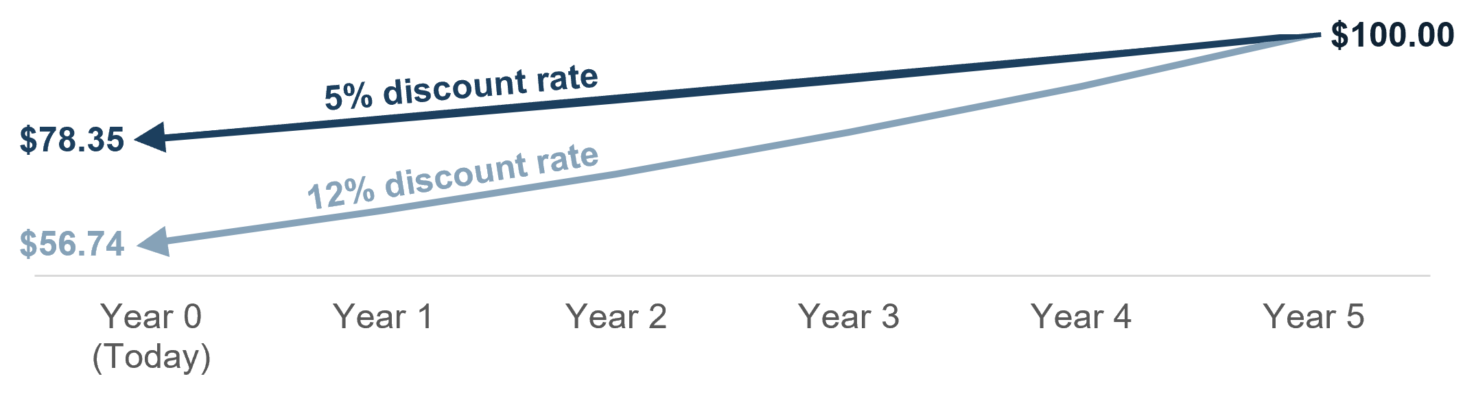
To show how this formula works, let’s take a simple example. Suppose a contract guarantees us a single payout of $100 in five years.
If we use a conservative discount rate of 5%, the present value of that cash today is $78.35
But if the project carries more risk and we use a discount rate of 12%, that same $100 payout drops to a present value of $56.74 today
By waiting five years under a higher risk profile, the present value of our cash falls by over $21.
How Risk Dictates the Rate
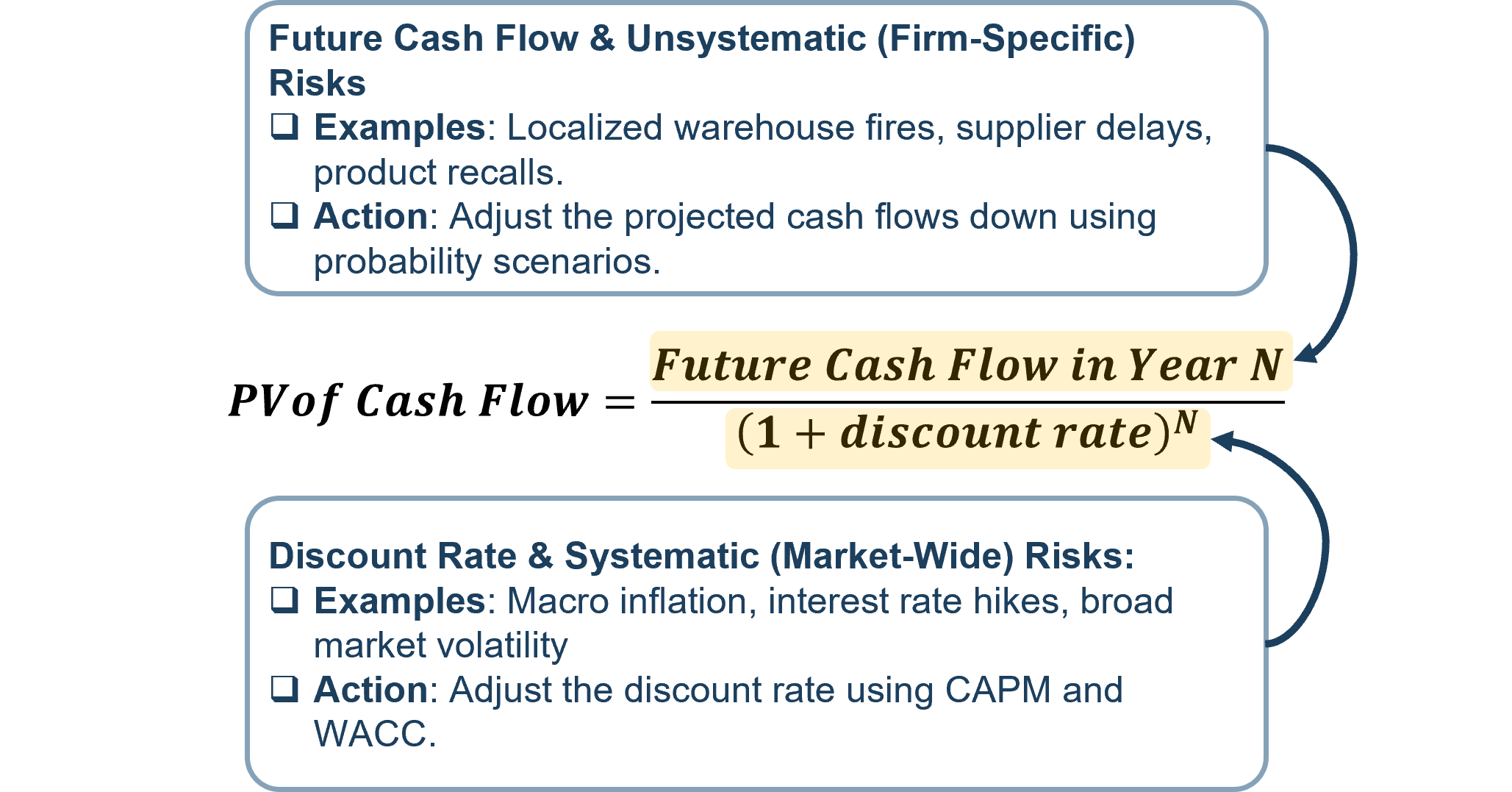
Why would our discount rate change from 5% to 12%? It comes down to how we categorize and handle risk. In finance, we divide risk into two distinct buckets:
Unsystematic Risk (Firm-Specific): This is risk unique to a single company or project, such as a localized warehouse fire, a supplier delay, or a product recall. We do not adjust our discount rate for these risks because a diversified investor can eliminate them by holding a portfolio of different stocks. Instead, we handle unsystematic risk in the numerator of our valuation model by adjusting our expected cash flow projections downward using probability-weighted scenarios.
Systematic Risk (Market-Wide): This is macroeconomic risk that affects the entire market, such as broad inflation, supply chain disruptions, or interest rate hikes. Because investors cannot diversify away from systematic risk, they demand a premium to bear it. This risk is priced directly into the denominator of our model—the discount rate.
Quantifying Risk in the Cost of Capital
To calculate the cost of equity (the return equity investors demand for bearing systematic risk), we use the Capital Asset Pricing Model (CAPM)

Let’s walk through each component here:
The risk-free rate rf is typically the yield on a 10-year U.S. Treasury bond (~4.7% today)
The expected market risk premium (rm— rf ), also called market return over the risk -free rate, would be the historical market return less the risk-free rate (~4.5% for the US)
The beta (β) measures how sensitive our specific stock is to macroeconomic swings (ranges from about -2.0 — +2.0, where 1.0 would be matching the broader market exactly)
The beta is the main variable that changes depending on our target company or target industry. For instance, a defensive utility business might have an equity beta of 0.60, meaning its stock is highly stable. On the other hand, a capital-intensive manufacturing or defense business might carry a beta of 1.50. This means if the broader market moves up or down by 10%, that company’s stock historically swings by 15%. Because of this heightened systematic volatility, CAPM mathematically forces the cost of equity higher to compensate investors.
If you would like to explore and compare equity betas by industry, Dr. Aswath Damodaran from NYU hosts an excellent database on his page.
Calculating WACC
Once we know our cost of equity, we blend it with our cost of debt to find the company’s overall discount rate. We use the Weighted Average Cost of Capital (WACC) formula:

Where:
The current market value of the company’s equity is weighted by the cost of equity we derived from the CAPM equation.
The current market value of the company’s debt is weighted by the company’s current cost of debt (typically found by looking at the most recently reported interest expenses) and the corporate marginal tax rate. Since interest payments on debt are tax-deductible, the formula reduces the cost of debt by (1 − tax rate) to account for this corporate tax shield.
If the company has preferred stock, the preferred shares would be included as another term and treated separately from the common equity, since preferred shares have a guaranteed dividend yield.
From the formula, we can tell that the value of equity (the stock price and outstanding shares) and the value of debt (especially if the company issues public bonds) will have a significant impact on the WACC. To see how capital structure shifts WACC in practice, let’s look at a quick example.
Suppose a company has a Cost of Equity (requity) of 10%, a pre-tax Cost of Debt (rdebt) of 6%, and a marginal tax rate (t) of 25% (making the after-tax cost of debt 4.5%).
Scenario A: 100% Equity / 0% Debt
If the company is entirely funded by equity, its WACC is simply equal to its cost of equity: WACC= (1.0 × 10% ) + ( 0.0 × 4.5% ) = 10.0%
Scenario B: 70% Equity / 30% Debt
If the company shifts its capital structure to include 30% debt, we blend the two costs: WACC = ( 0.70 × 10% ) +( 0.30 × 4.5% ) = 7.0% + 1.35% = 8.35%
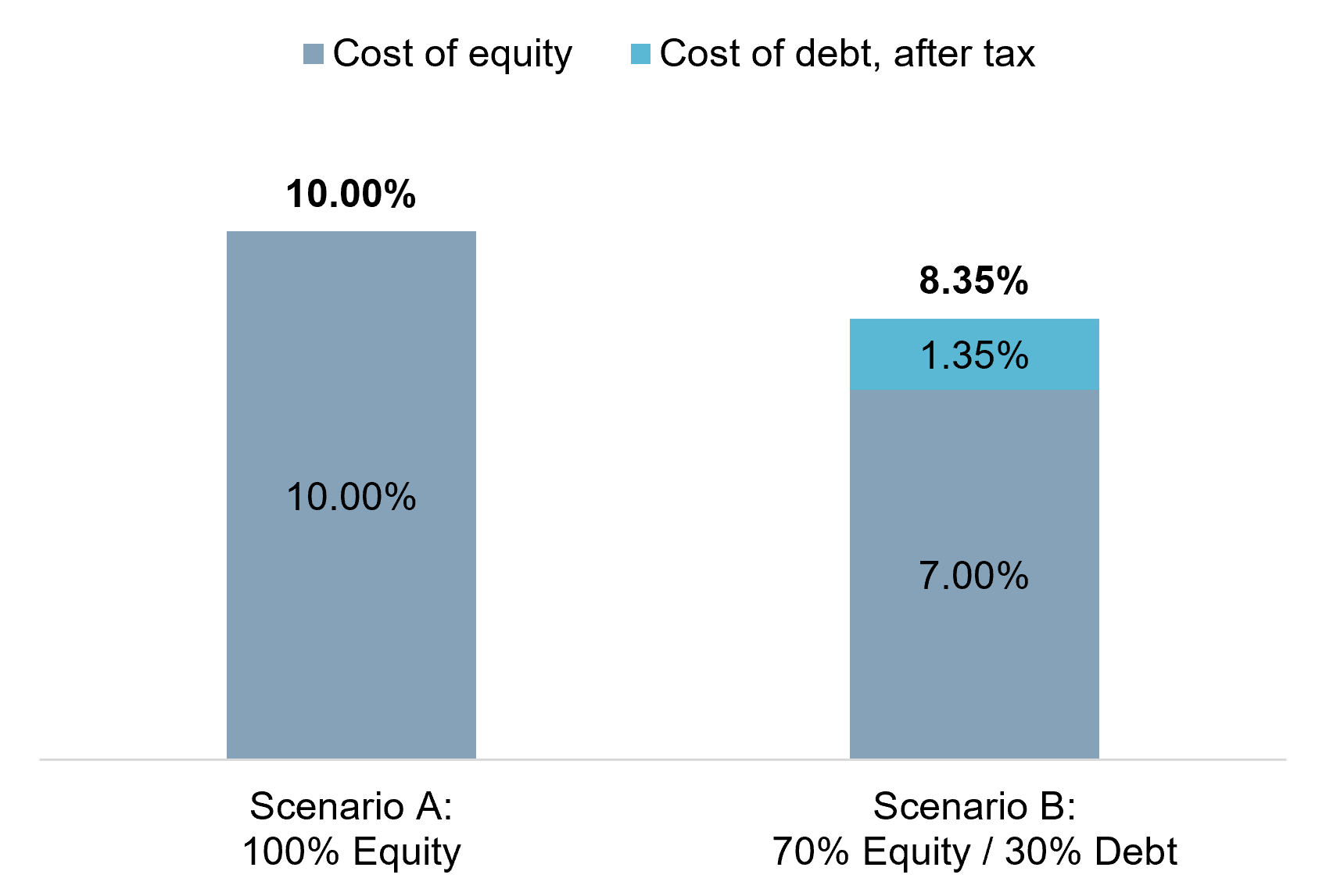
By introducing cheaper, tax-shielded debt into the capital structure, the company lowers its overall WACC from 10.0% to 8.35%. In a valuation model, lowering the discount rate (the denominator) increases the present value of the company’s future cash flows, so executives consider how to fund business investments based on this dynamic.
Key Takeaway
In practice, analysts will run a range of scenarios with different assumptions for discount rates or cash flow projections. The scenarios are based on company-specific or market-driven “What ifs” like “what if it takes six months longer to start up that new factory?” or “what if interest rates change next year?” These factors will impact the present value of an investment and scenarios modeling can help leaders better understand what is at stake and whether a new project still makes sense to pursue.
Ultimately, financial valuation is not about predicting the future with absolute certainty. It is about understanding these risk dynamics so we can translate future uncertainty into clear, logical investment decisions today. We can model or quantify that risk by considering whether a specific risk is firm-specific (unsystematic) or market-wide (systematic) and adjusting our cash forecast or discount rate appropriately.
© Katherine Dextraze, F Avenue Consulting, 2026
Great breakdown of TVM and the distinction between handling systematic risk in the denominator and unsystematic risk in the numerator!
I particularly liked how clear you made the capital structure dynamic with WACC. One minor thought to add on the practical side: while tax-shielded debt initially drives down WACC, there’s always that delicate tipping point where financial distress costs and bankruptcy risk kick in, causing both equity and debt holders to demand higher returns and driving WACC back up.
Thanks for sharing such a crisp, structured overview!